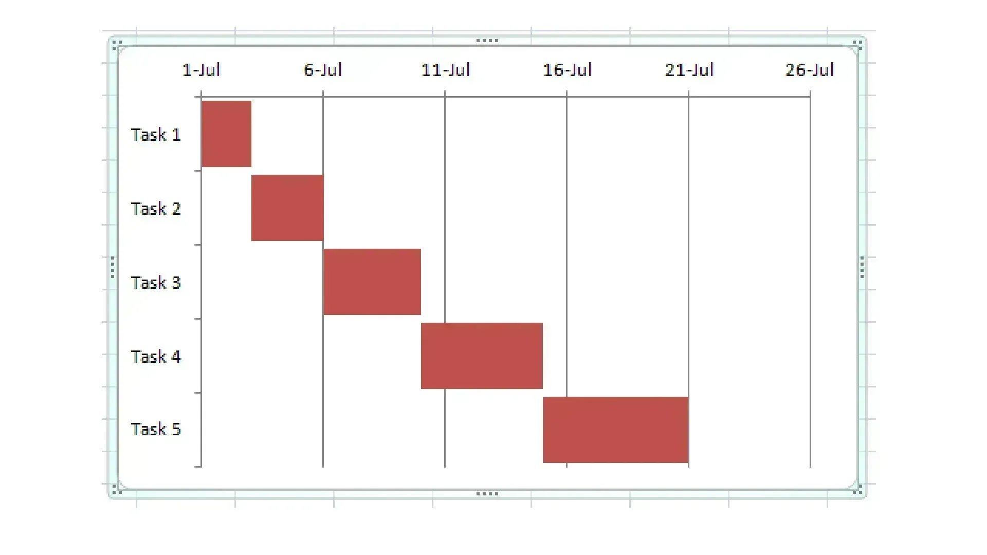
How To Create Gantt Chart In Excel Less Than Four Minutes

Microsoft Excel does not specifically offer the option to create Gantt charts. Fortunately, it is still possible to create Gantt chart in Excel with some creativity and some insight into how the program works.

What is A Gantt Chart?

From 1910 to 1915, engineer and scientist Henry L. Gantt worked to come up with a charting system that could be used to track and manage progress on projects. What he invented was a form of a bar chart. On the x-axis, he tracked time broken down into increments of days, weeks, months, or years. On the y-axis, he placed the series of tasks required for the successful completion of the project. Using a series of bars, he could track when each task should be started and when it should be completed over the lifetime of the project.

These relatively simple charts are still in use because they intuitively lay out the plan for even the most complex projects. Despite being invented more than 100 years ago, Gantt charts continue to be an efficient form of project management, which is why being able to create one in Excel is such a useful skill.

Create A Gantt Chart In Excel

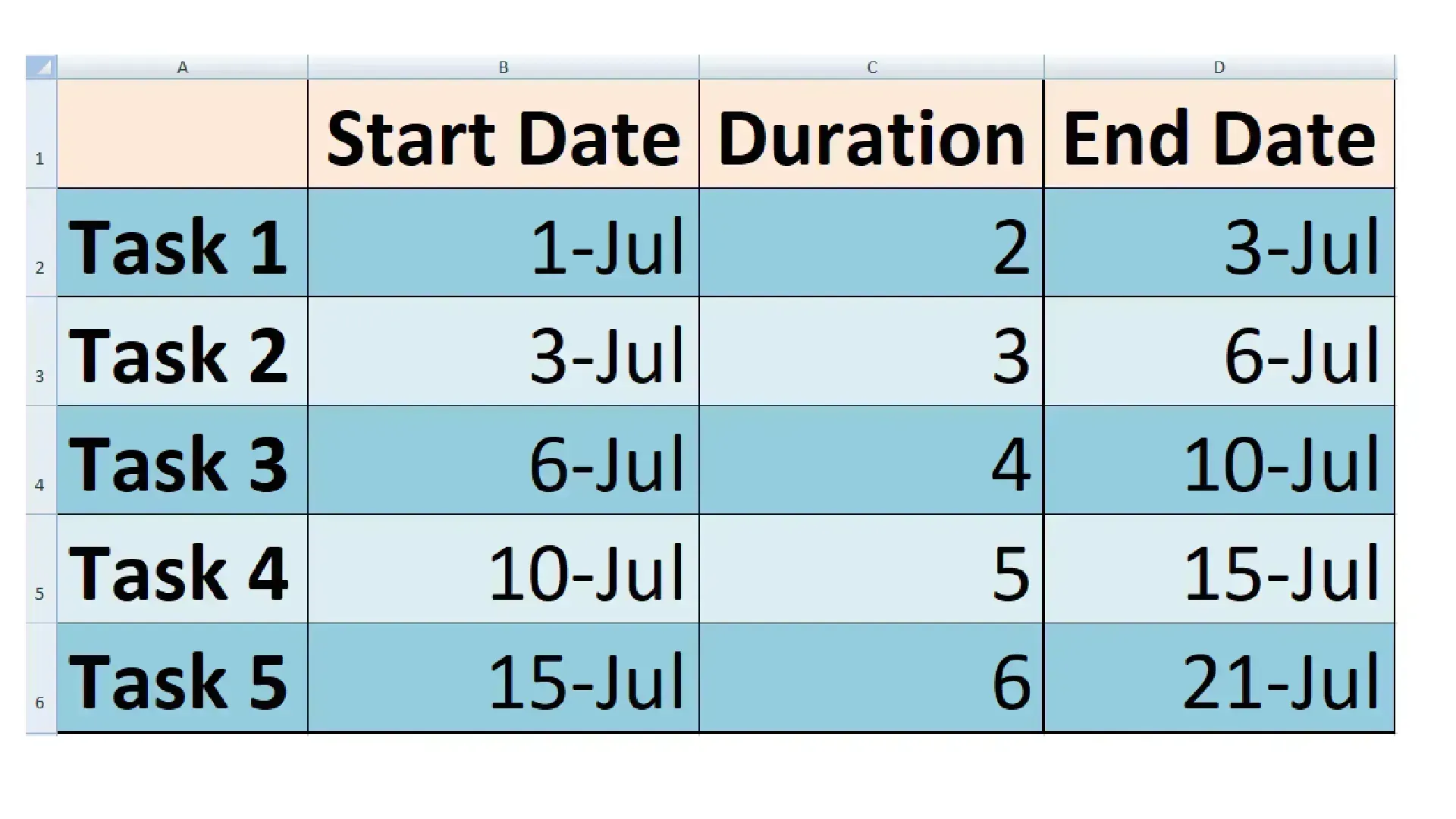
Step One: In order to create a Gantt chart in Excel, there are a few pieces of information that you need to have: a list of tasks to be completed, a start date for these tasks, the date by which each task needs to be complete, and the duration of each task. Once you have this information, create an Excel table. It is important to make sure that the information you have is complete and accurate because what you have in your table is exactly what you will used to create your chart.

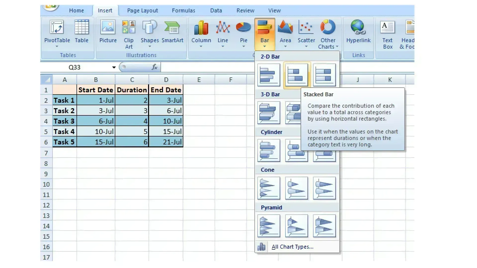
Step Two: Convert your worksheet into a bar chart by clicking on the following: Insert, Bar, and Stacked Bar. This will cause a blank box to appear on your worksheet.

Step Three: Right click on the empty box. Left click on Select Data, which will open the Select Data Source window.

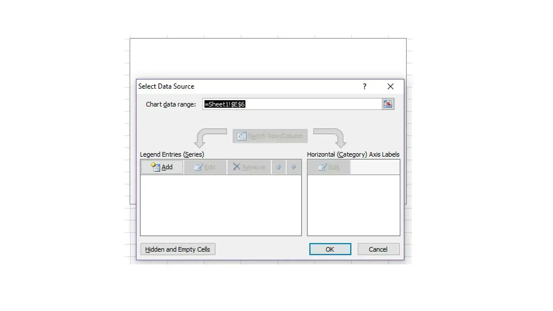
Step Four: In this menu, select Add. Click on Series name, and click on the table cell that reads Start Date. Click on the icon next to Series values that looks like a small spreadsheet, which will open the Edit Series window. Highlight all of the cells from the first Start Date to the last Start Date by dragging your mouse over the cells.

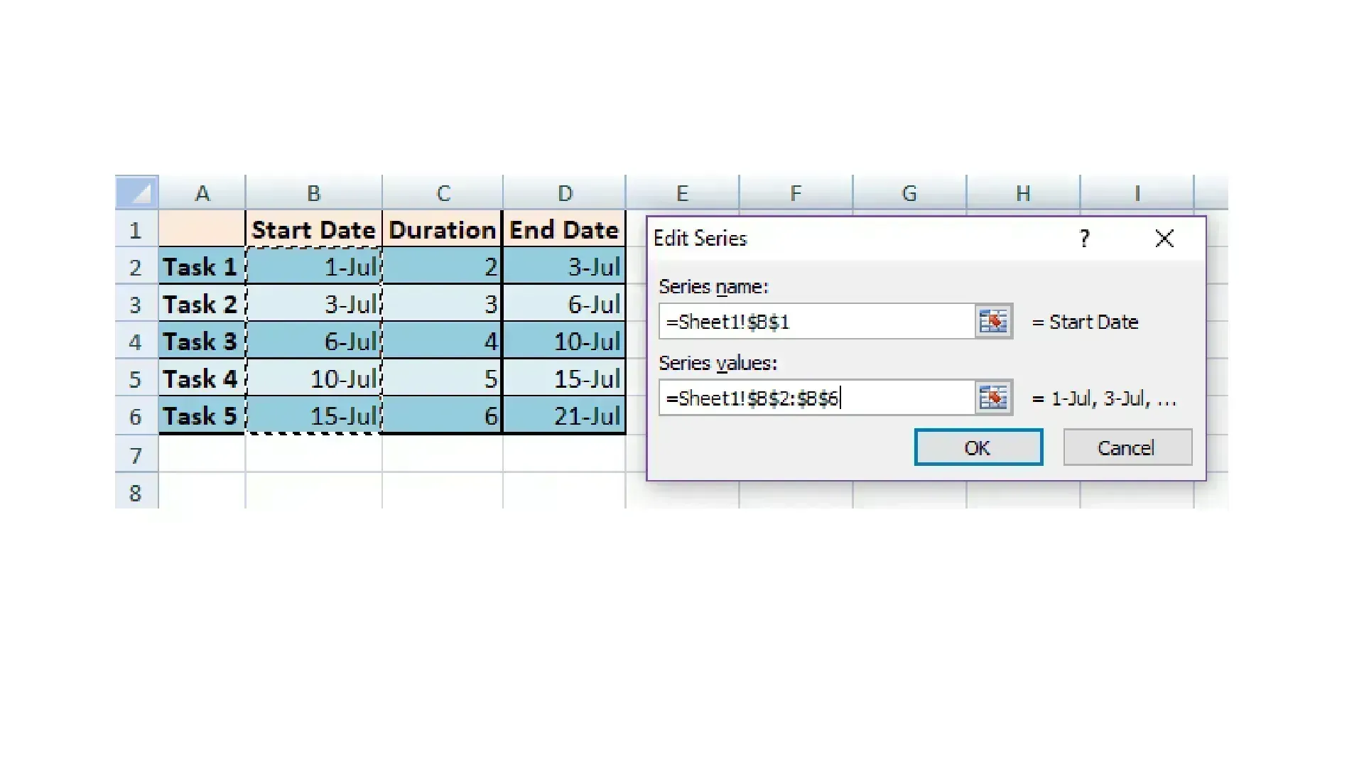
Step Five: Click on the small spreadsheet icon to return to the previous window, and click OK. The information will appear on your chart in a series of bars. Repeat this process using the Duration column. You now have all of the information you need on your chart.

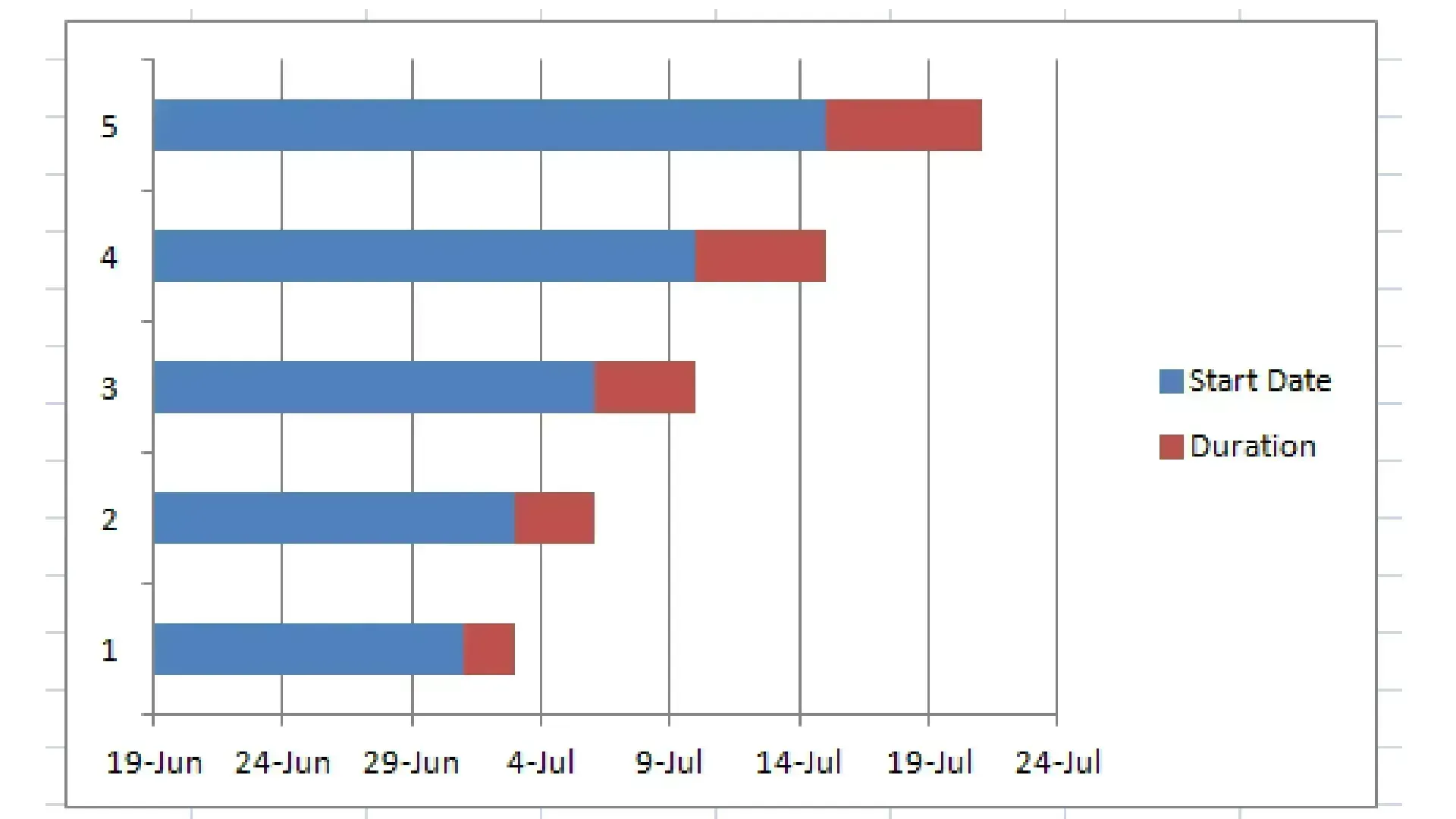
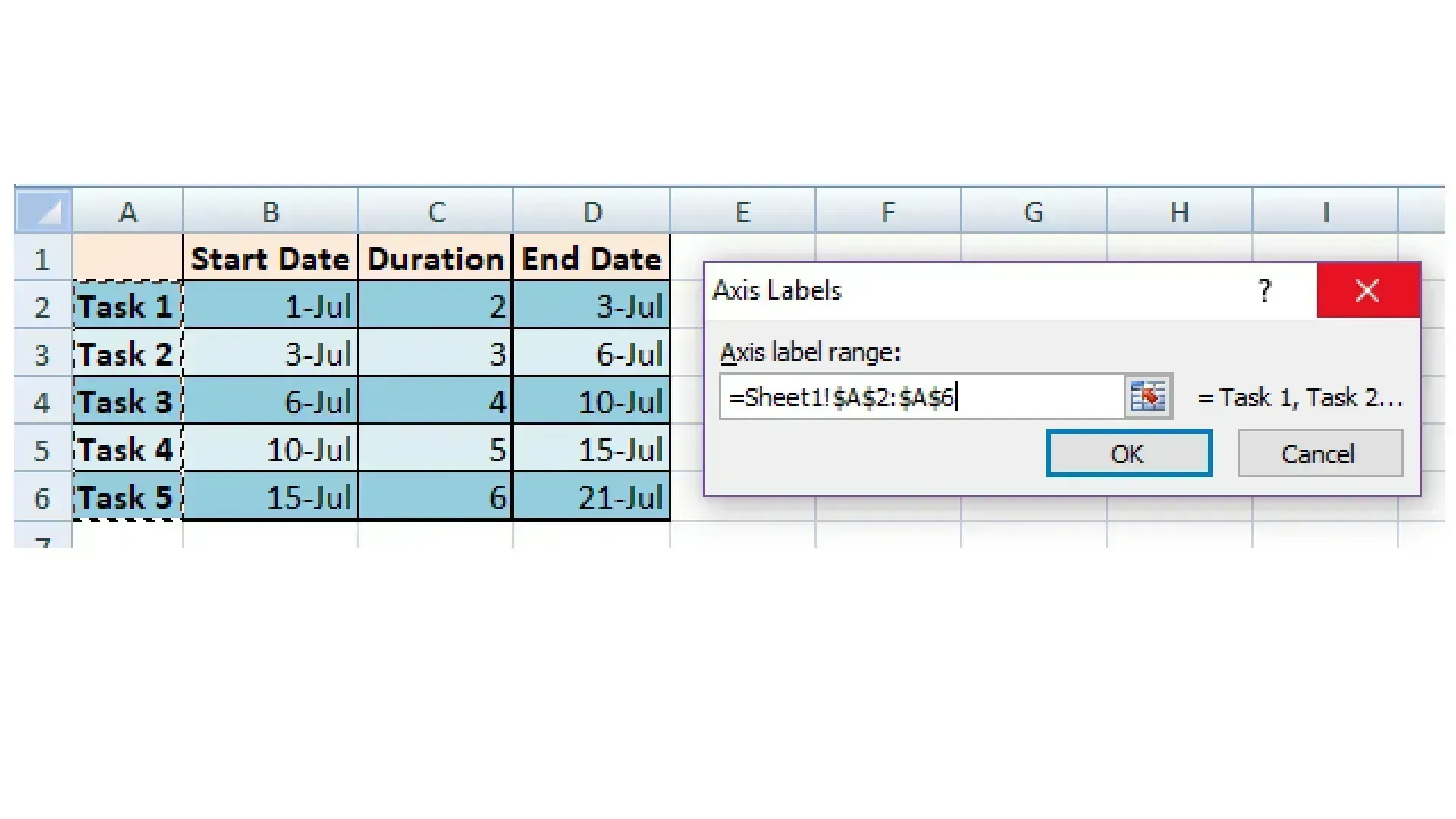
Step Six: Change the left column labels to match the names of each task. To do this, click on any bar in the chart. Then, right click on it. Click on Select Data, and select Edit under Horizontal (Category) Axis Labels. Highlight the list of tasks by dragging your mouse over them, and click OK twice.

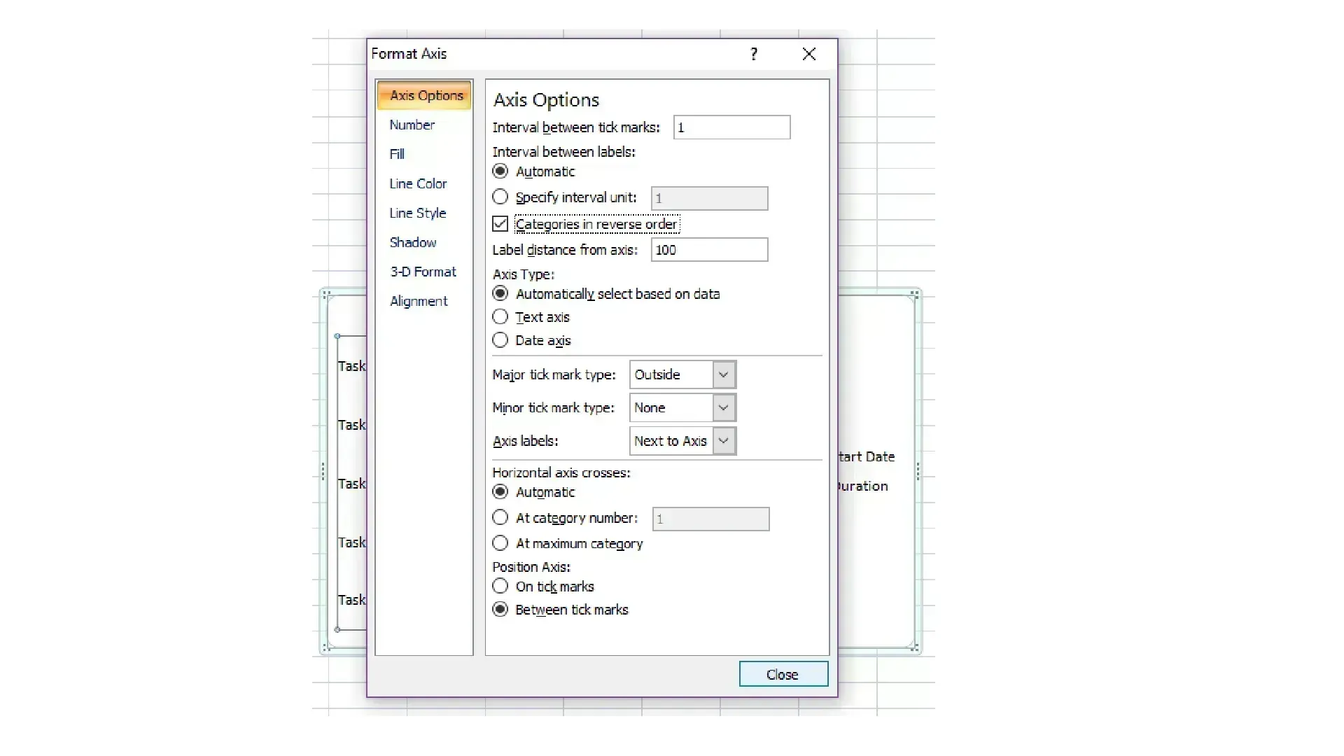
Step Seven: You will notice that the list of tasks on your chart is in reverse order. To correct this, right click on the list of tasks. Select Format Axis, and check the box next to Categories in reverse order.

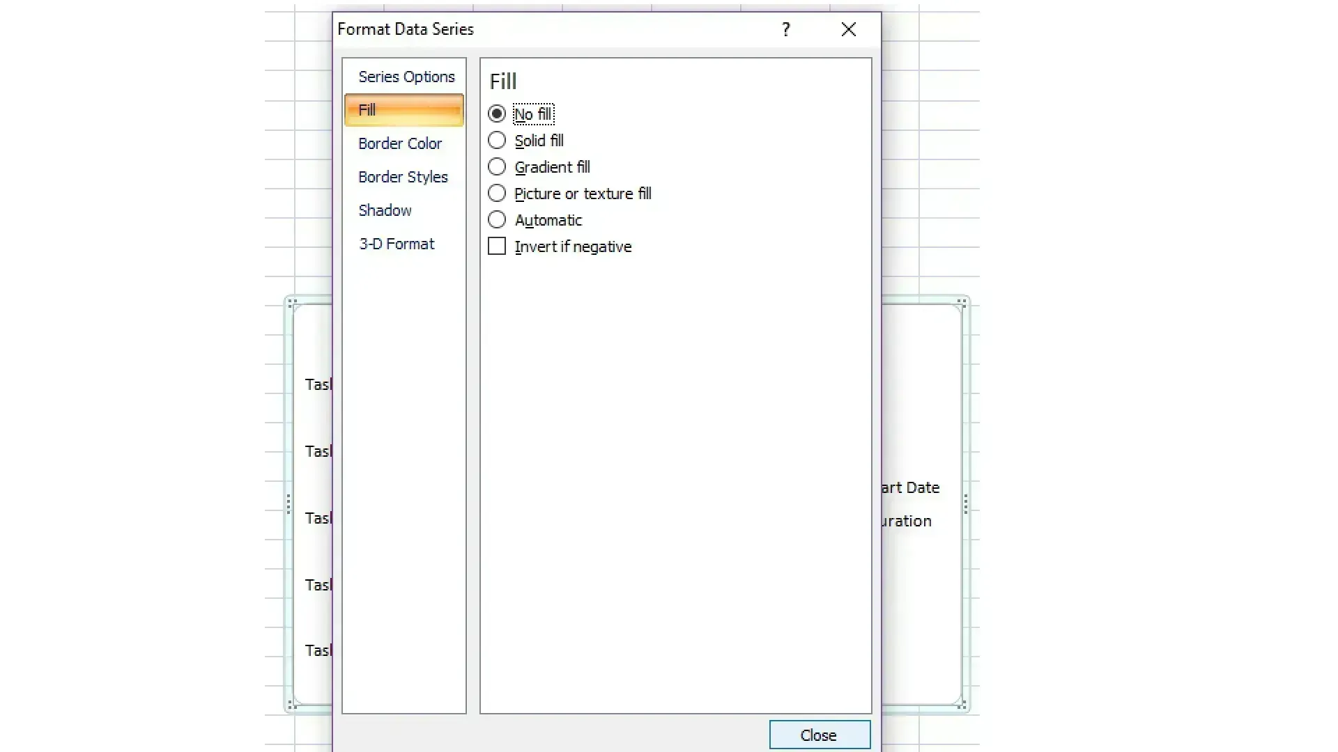
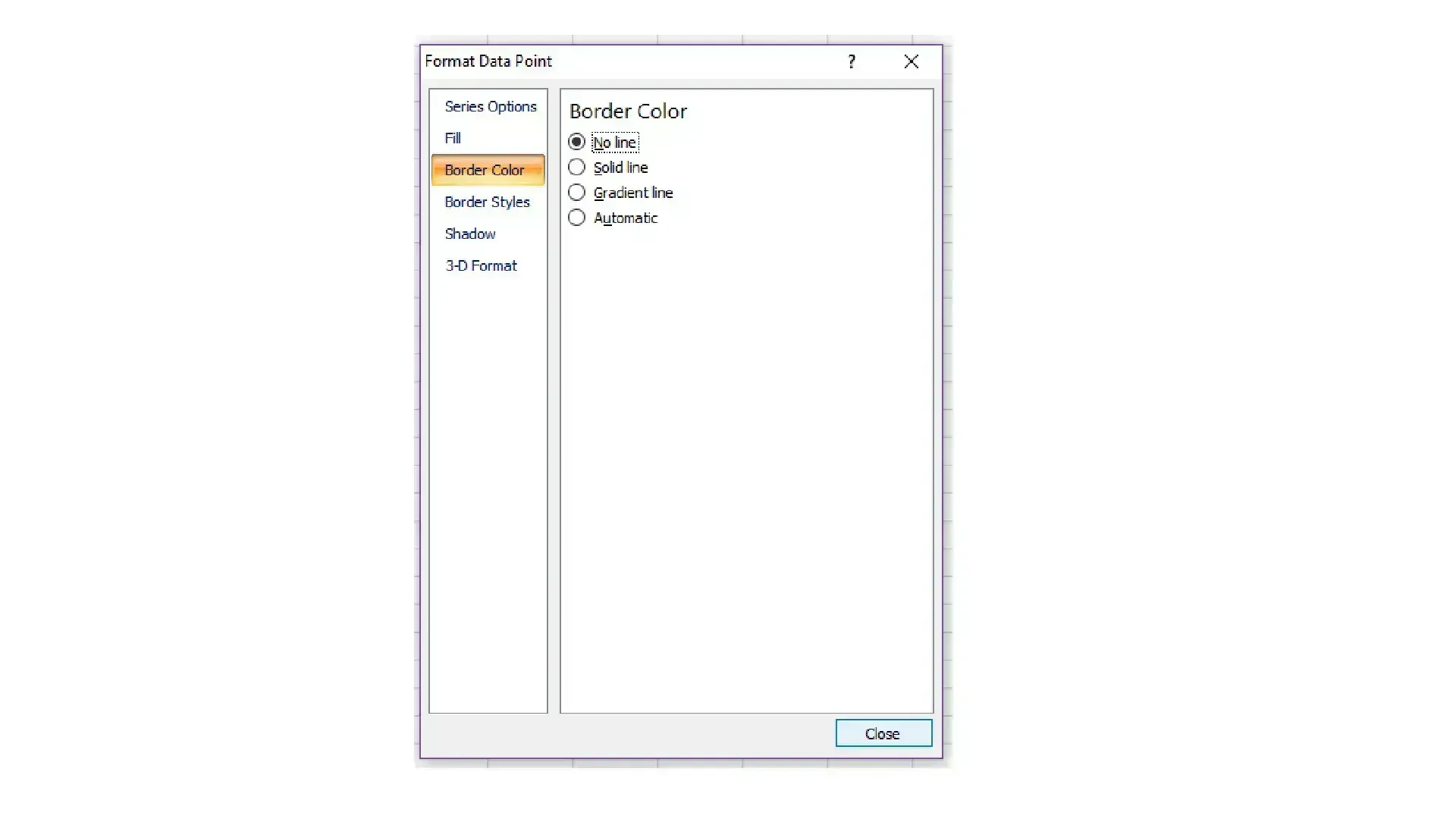
Step Eight: Remove the blue portions of each bar on the chart. Select the blue section of any bar, right click on it, and select Format Data Series. In this window, go to the Fill menu, and select the No fill option. Also, go to the Border Color menu, and select No line.

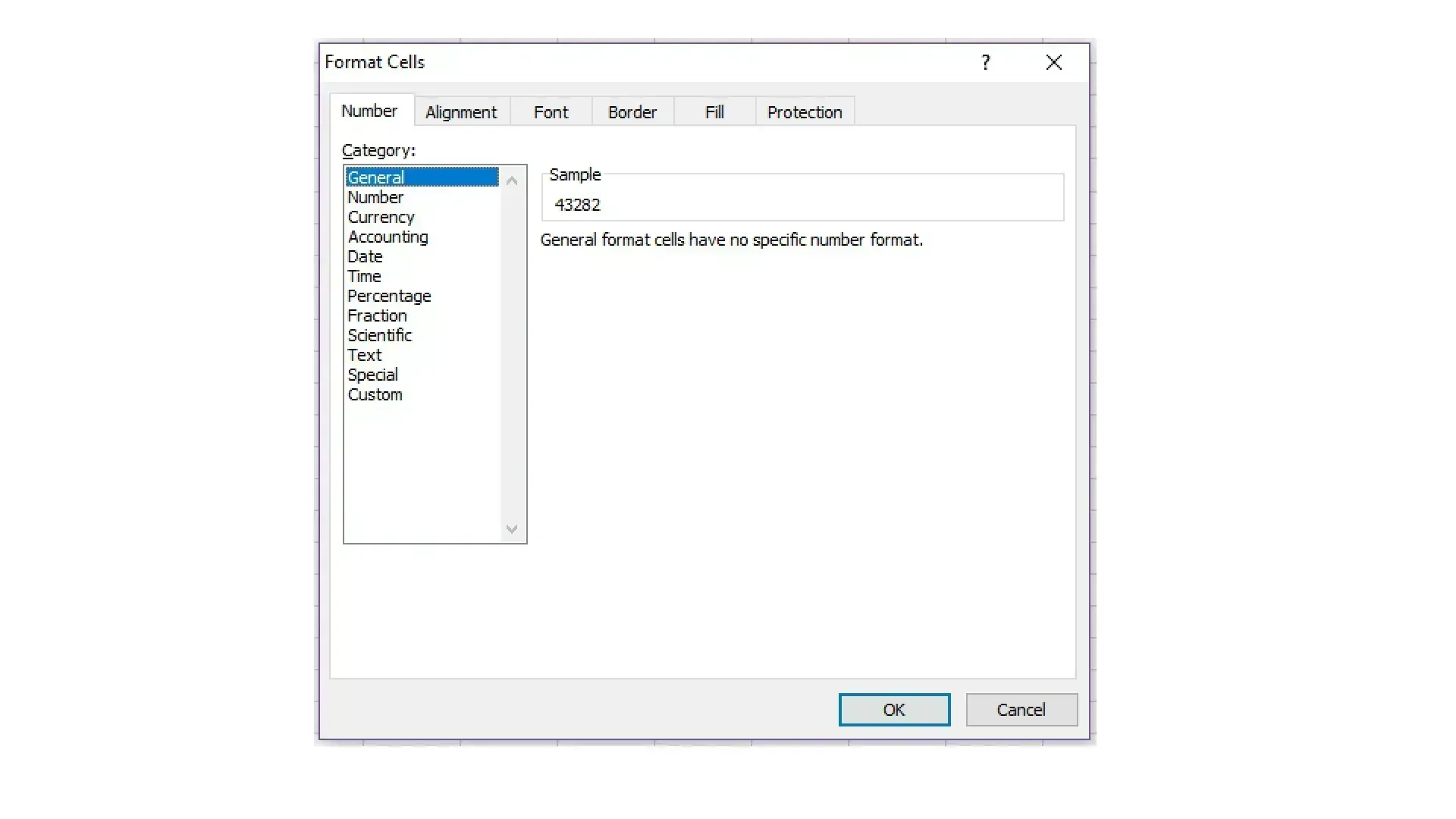
Step Nine: Fix the innacurate dates along the horizontal axis. Go to your original spreadsheet, right click on the start date of the first task, and select Format Cells. Under the Number tab, click on General. Record the number you see under Sample, and exit the window. Keep in mind that this number varies, so it doesn't matter what the number actually is.

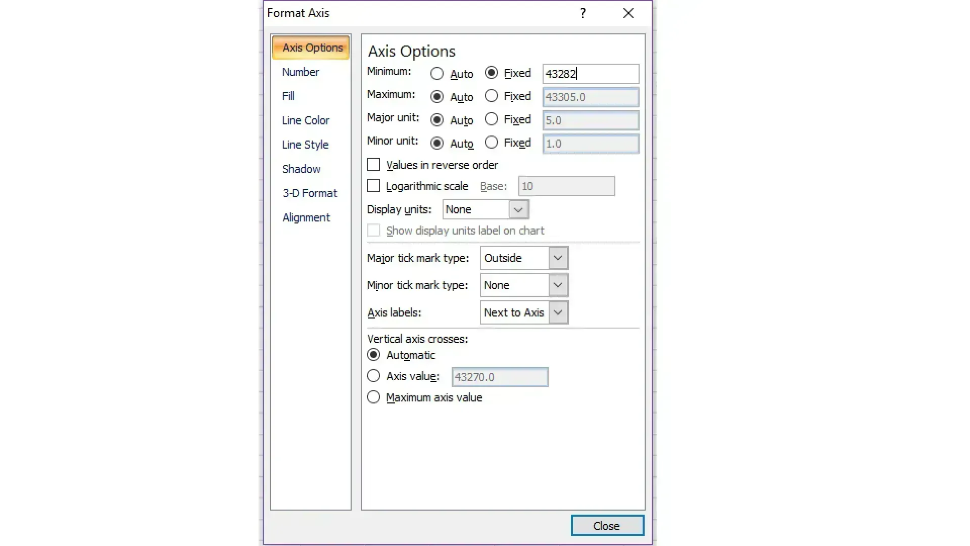
Step Ten: On your chart, click on the dates to select them, right click on them, and select Format Axis. Go to the Axis Options menu, click the Fixed option next to Minimum, and type in the number you recorded earlier.

Bonus Tips and Tricks: To create more space for your chart, you can get rid of the legend. Simply click on it, and delete it. You can also get rid of some of the excess white space on the chart. Click on any bar, select Format Data Series, and go the Series Options menu. Set Series Overlap to 100% and Gap Width to 10%. You can also experiment with these numbers to see which settings work best for your specific chart.

It's that easy! By following these simple steps, you're able to create Gantt chart in Excel, and you're also able to customize the chart to meet your specific needs and goals.